The Physics of Racing,
Part 28: Hazards of Integration

Brian Beckman, PhD

©Copyright December 2001

The equations of motion are differential equations. Such equations tell us how to calculate "what's happening now" from "what happened a little while ago." They're called differential because they have the form of ratios of differences (qua subtraction or differentiation or derivatives) between "what's happening now" and "what happened a little while ago." The process of solving the equations, that is, finding out "what's happening now," is integration, a kind of addition, which reverses the subtraction of differentiation. In computer simulation, we integrate numerically, but numerical integration is fraught with hazards. In this article, we give a stark illustration of a very simple differential equation going massively haywire under a very straightforward integration technique. We also introduce MATLAB (from www.mathworks.com) as a programming, visualization, and design tool.

As usual, let's start with Newton's Second Law (NSL), F = ma. Acceleration, a, is the rate of change or first derivative of velocity, which is how much velocity changes over a small interval of time. Consider the following chain of definitions:

The first term says "acceleration at time t = t₂ is the ratio of the difference of the velocities at two times ("now," t₂, and "a little while ago," t₁), divided by the difference of the two times, calculated as we push the two times closer and closer." The velocity differences will get smaller and smaller, but the time differences will get smaller and smaller, too, so the ratio will, one hopes, converge to a certain number, and we call that number the acceleration. If the acceleration is large, the velocity will be changing quickly over short times, so the difference v(t₂) - v(t₁) will be large compared to t₂ - t₁. We gloss over lots of detail, here. If you need a refresher, let me suggest looking up "differential calculus" on www.britannica.com.

We can see that "what's happening now," namely v(t₂) depends on "what happened a little while ago," namely v(t₁), and on mass m and force F. Likewise velocity is the rate of change of position, v = dx/dt. So, just as the velocity now depends on the velocity a little while ago through the acceleration, the position now depends on the position a little while ago through the velocity. We use two, linked, first-order differential equations to get position.

Numerically, as in simulation, we cannot actually collapse the two times. That's only possible in a symbolic solution, also called exact, closed-form, or analytic. Rather, in a typical simulation setting, , the integration step size, will be set by the environment, often by a graphics rendering loop. At 30 frames per second, an acceptable minimum, will be about 33.3 milliseconds (msec) or 1/30 seconds. At 100 miles per hour, or 147 feet per second, a car will go about feet in that time. This means that with an integration step size of 33 msec, we can only predict the car's motion every five feet at typical racing speeds. This back-of-the-envelope calculation should make us a little nervous.

To find out how bad things can get, we need an example that we can solve analytically so we can compare numerical solutions to the exact one. A whole car is far, far too complex to solve analytically, but we usually model many parts of a car as damped harmonic oscillators (DHOs), and a DHO can be solved exactly. So this sounds like a highly relevant and useful sample.

In fact, it turns out that we can get into numerical trouble with an undamped oscillator, and it doesn't get much simpler than that. So, consider a mass on a spring in one dimension. The location of the mass is x(t), its mass is m, the spring constant is k, and the mass begins at position x(t = 0) = x₀ and velocity v(t = 0) = 0. Hooke's Law tells us that the force is -kx(t), so the differential equation looks like

The process for solving differential equations analytically is a massive topic of mathematical study. We showed one way to go about it in Part 14 of the Physics of Racing, but there are hundreds of ways. For this article, we'll just write down the solution and check it.

is the angular frequency in radians per second, or the reciprocal of the amount of time the oscillator's argument takes to complete 1 radian of a cycle. Since there are radians in a cycle, the period of the oscillator, or the amount of time to complete a cycle, is [seconds per cycle = radians per cycle/radians per second].

Let's plot a specific example with numbers picked out of a hat: m = 10kg, or about 98 Newtons or 22 lbs k = 1 N/m. We expect the period to be or almost 20.

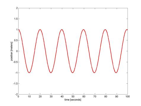
Sure enough, one cycle of the oscillator takes about 20 seconds. We used MATLAB to generate this plot. This is an interactive programming environment with matrices as first-class objects, meaning that pretty much everything is a matrix. We first set up a 1-dimensional matrix, or vector, of time points

Read this as follows: h is a (scalar) time step equal to 0.1 seconds tn is an upper bound (scalar) equal to 100 seconds tt is a vector beginning at time 0, ending at time tn, and having a value every h seconds. tt has 1001 elements, namely 0.1, 0.2, 0.3, ..., 99.9, 100.0. Sample the solution, , at these points and plot it with the following commands:

The string '-r' means 'use a straight red line'. The only other notation that might not be obvious in the above is the argument of axis, namely [0, tn, -2 2]. This is an explicit or literal vector of limits for the axes on the plot. It's a little strange that the axis limits and the labels are specified after the plot command, but that's the way MATLAB works. Note that the missing comma between -2 and 2 is not a typo: commas are optional in this context.

Now that we know what the exact solution looks like, let's do a numerical integration. Not long after the differential calculus was invented by Liebniz and Newton, Leonhard Euler articulated a numerical method. It's the most straightforward one imaginable. Suppose we have a fixed, non-zero time step, . Then we may write an approximate version of the equation of motion as . If we know x(t) and v(t), position and velocity at time t ("a little while ago"), then we can easily solve this equation for the unknown , velocity now namely . Likewise, we approximate the position equation as , or . With these two equations, all we need is x(0) and v(0) and we can numerically predict the motion forever. Here's the MATLAB code:

The first thing to note here is that we've packaged up position and velocity in another vector. This is very convenient since MATLAB prefers vectors and matrices, and it's possible because both equations of motion are first-order by design, that is, they each contain a single, first-derivative expression. We then integrate this pair of equations by calling euler with a function name in a character string, the time a little while ago, the solution vector a little while ago, and the integration step size, here written h. Here's euler:

Euler builds up a string from the function name and its arguments, calls the function via the built-in eval instruction, then updates the solution vector and the time and returns them in a new vector. The eval instruction is the equivalent of calling a function through a pointer, which should be a familiar concept to C++ programmers. Here's the function we call:

The function models the pair of differential equations by a matrix multiplication. In traditional notation, here's what it's doing:

, or

A few moments' thought should convince anyone still with us that the MATLAB code is doing just what we want it to do. Let's plot:

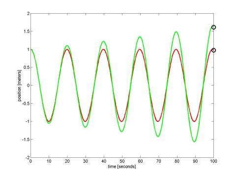
DISASTER! The numerical version is 60% larger than it should be at 100 seconds, and looks as though it will continue to grow without bound. What could be wrong? Let's look back at our approximate equations.

What would happen if a small error, say , crept into the velocity? Instead of the above, we would have, at the first step,

The predicted velocity, , will be in error by and the position by . If no further errors creep in, what happens at the next step?

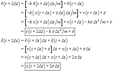
The position error gets WORSE, even when no further errors creep into the velocity. The velocity errors might not get worse as quickly much depends on the size of relative to . However, working through another step, we can conclude that

so the velocity errors will eventually overwhelm as grows.

What is to be done? The answer is to use a different numerical integration scheme, one that samples more points in the interval and detects curvature in the solution. The fundamental source of error growth in the Euler scheme is that it is a linear approximation: the next value depends linearly on the derivative and the time step. But it is visually obvious that the solution function is curving and that a linear approximation will overshoot the curves.

In this article, to keep it short, we simply state the answer and demonstrate its efficacy. The 4^th-order Runge-Kutta method is the virtual industry standard. In a later article, we intend to present an original derivation (done without sources for my own amusement, as is usual in this series), if the length turns out to be reasonable and level of detail remains instructive. This method samples the solution at four points interior to each integration step and combines them in a weighted average. For now, take the location of the interior sample points and the magnitudes of the averaging weights on faith: they're the subject of the upcoming derivation. In the mean time, you can look up various derivations easily on the web. Here's the cookbook recipe: for full generality, rewrite the equation as a derivative's equalling an arbitrary function of time and the solution (this is much more general than our specific case):

Then, chain solution steps to one another as follows:

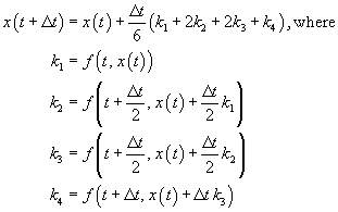
This is a lot easier to implement than it looks, especially when we rewrite the old Euler scheme in a similar fashion

and when we show the MATLAB code for it:

Make a plot exactly as we did with Euler, in fact, let's plot them both on top of each other in a 'movie' format along with the exact solution (it's only possible to appreciate the animation fun, here, if you have a running copy of MATLAB):

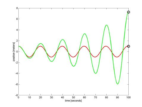
In the following plot, we show the results of running the code above with changed to 0.4 from 0.1, showing how the errors in euler accumulate much faster over the same time span (we also adjusted the axis limits for the larger errors). The most important thing to notice here is how the Runge-Kutta solution remains completely stable and visually indistinguishable from the exact solution while the Euler method goes completely mad.

More info