In this instalment, we revisit the four-wheel statics of Part 20, solving the statics problem for level ground, which is very common in simulation. The problem is: given lateral and longitudinal forces, find the balancing vertical forces. In so doing, we introduce a conventional coordinate system and a new tool: Mathematica. This is a comprehensive mathematics package that we use for symbolic manipulation.
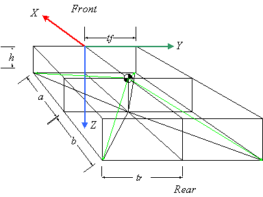
First, let's introduce the standard coordinate frame used by the SAE, which is documented in the usual source books by Milliken (Race Car Vehicle Dynamics) and Gillespie (Fundamentals of Vehicle Dynamics). In this frame, X is forward (longitudinal), Y is to driver's right (lateral), and Z is downward (vertical), in the direction of gravitation. The following figure illustrates:

The symbols have the following meanings:
| h | vertical distance of the Centre of Gravity (CG) from the ground |
| a, b | longitudinal distance from the CG to the front and rear axle geometry centres |
| tf, tr | front and rear half-track lateral distances from axle centres to contact patch (CP) |
These give us the geometry needed to locate the CPs. Let's code this up in Mathematica (MMA, see http://www.wolfram.com/). We open up an MMA 'Notebook' and write
tyreLocs = {{a, tf, h}, {-b, tr,
h},
{-b, -tr, h}, {a, -tf, h}}
This code defines tyreLocs as a list of 3-vectors, each being a list of locations in three-dimensional space in the car-fixed, SAE coordinate frame. Numbered the tyres clockwise from right front (RF). So the RF tyre has location X = a, Y = tf, and Z = h, and so on for the RR, LR, and LF, in order. Note that a, tf, and h do not need predefined values: MMA treats any undefined symbol as just a symbolic constant (nice!). This is the distinguishing aspect of a symbolic math language like MMA as opposed to an ordinary computer language like C++.
Define a numerical sample early so that it's handy for intuitive checks. The following are for a Lamborghini Diablo, found from a web search, in Meters and Newtons:

This code defines a variable, numRz, whose value is a list of MMA rules. The following function of two parameters shows how to apply rules:
num18 [term_, fRzInput_] := ((term /. numRz) /. fRzInput)
This code defines a function named nml8 that takes any term and applies to it first the rules numRz and then any other set of rules, locally named fRzInput. The underscores after the names term and fRzInput in the parameter list are part of MMA's deep pattern-matching syntax. For present purposes, just think of them as necessary noise when defining a function. Test what we have so far as follows:
nm18 [tyreLocs, {}]
{{1.425, 0.8675, 0.42}, {-1.029, 0.88,
0.42},
{-1.029, -0.88, 0.42}, {1.425, -0.8675, 0.42}}
Here is see an example of input and output syntax from MMA. We applied the function nml8 to the pre-existing list of geometry vectors and to a null list of extra rules to get numerical locations of the CPs. These numbers are sensible, by inspection.
Now make a couple of symbolic lists of forces operating on the tyres. Separate the forces operating in the X - Y plane from the vertical forces since the former are given and the latter are the final objects of our solution efforts.
| fxy =
{ {f1x, f1y}, {f2x, f2y}, (* right side *) {f3x, f3y}, {f4x, f4y}} (* left side *) fz = {f1z, f2z, f3z, f4z} |
For immediate purposes, combine them into three-forces, and there is some magic juju for doing that in MMA:
threeForces = MapThread [Append, {fxy, -fz}]
{{f1x, f1y, -f1z}, {f2x, f2y, -f2z}, {f3x, f3y, -f3z}, {f4x, f4y, -f4z}}
Lisp programmers will say " Aha!" MapThread runs a function, in this case, Append, down some lists, and Append glues lists together. The two threaded lists are fxy and fz, defined immediately above. Use the negative of fz so that the vertical force vectors point upwards and the force components can be positive numbers. This code makes a new list of four 3-forces named threeForces.
Now to the physics. Remember that torque is lever - arm  force, where
  is the vector cross product. We have
lever-arms in one list, tyreLocs, and
forces in another, threeForces, so the
torques about the CG at each CP are immediately available:
threeTorques = MapThread [Cross, {tyreLocs, threeForces}]
{{-f1y h - f1z tf, a f1z + f1x h, a f1y -
f1x tf},
{-f2y h - f2z tr, -b f2z + f2x h, - b f2y - f2x
tr},
{-f3y h + f3z tr, -b f3z + f3x h, -b f3y + f3x
tr},
{-f4y h + f4z tf, a f4z + f4x h, a f4y + f4x
tf}}
When the car is not flipping over, the X and Y torques are in equilibrium. The Z torque accounts for yaw, so it's free. Add up the X and Y torques:
sumTorques = Simplify [Plus @@ threeTorques]
{{-f1y h - f2y h - f3y h - f4y h - f1z tf +
f4z tf - f2z tr + f3z tr,
-b (f2z + f3z) + a (f1z + f4z) +
(f1x + f2x + f3x + f4x) h,
-b (f2y + f3y) + a (f1y + f4y)
- f1x tf + f4x tf - f2x tr + f3x tr}
" @@" is MMA juju for applying the function Plus across a list of vectors. It's similar to MapThread, but not quite the same (see the MMA documentation for details). Construct and solve the X and Y equations for torque equilibrium:
torqueEquations = {sumTorques[[1]] == 0, sumTorques[[2]] == 0}
The double square brackets pick out elements of lists, so sumTorques[[1]] is the first element of sumTorques, that is, the torque about the X axis. The double-equals is an assertion that sumTorques[[1]] is zero, and solvable MMA equations must contain double equals. We have a similar equation for sumTorques[[2]], the Y torque. Thus, torqueEquations is a list of two equations. Solving:
rightHandRules = Solve [torqueEquations, {f1z, f2z}] // FullSimplify

This code solves the equations for the specified variables, f1z and f2z, expressing the solution as rules that can be applied in other contexts. We've already seen numerical rules in action, but we can have symbolic ones too, and equation solutions are an example.
These solutions are a 'mouthful', but notice, slightly surprisingly, that the lateral and longitudinal forces show up only as their sums, so reduce the amount of 'verbiage' by defining and applying a couple of rules by hand
fxRule = f1x + f2x + f3x + f4x fx
fx
fyRule = f1y + f2y + f3y + f4y fy
fy
rhr = rightHandRules /. {fxRule, fyRule}

lhr = leftHandRules /. {fxRule, fyRule}

Notice the solution for the left-hand side (LHS) of the car, obtained by methods analogous to those for the right-hand side (RHS). These expressions are much more digestible. The first thing to notice is that the solutions for f1z and f2z, on the RHS, depend on the solutions for f3z and f4z on the LHS. This is no help. As discussed in Part 20 of the Physics of Racing, we need more information. Posit that cross ratios of weights are equal: that any weight-jacking in the car is symmetric. For instance, the ratio of left to right is the same at front as at rear, or, equivalently, that the ratio of front to rear is the same on left as at right. These conditions yield another equation.
eq1 = f1z f3z == f2z f4z
Get one more equation from force equilibrium: the sum of all vertical loads equals the weight of the car.
eq2 = mg == (f1z + f2z + f3z + f4z)
Solve for rules to eliminate f3z and f4z from the right-hand rules obtained above:
s34 = Solve [{eq1, eq2}, {f3z, f4z}]

rTea = Flatten [FullSimplify [rhr /. s34]]
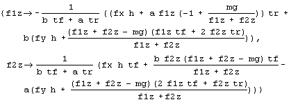
The important thing here is the expression rhr/.s34, which applies the elimination rules to rhr. The functions FullSimplify and Flatten are afterthoughts to reduce the verbosity of the symbolic results.
This is great. We have expressions that depend only on f1z and f2z, so we have successfully isolated the RHS. Convert these rules to equations thusly, and solve again:
rNoah = Map [Apply [Equal, #] & ,
rTea]
rSoln = Simplify [Solve [rNoah, {f1z, f2z}]]
sf1z =
rSoln [[1, 1, 2]]
sf1zs = FullSimplify [sf1z]

Some of the above, you must take on faith due to lack of space to explain. Suffice it to say that we do likewise for tyres 2, 3, and 4, getting
sf2zs = FullSimplify [sf2z]

sf4zs = FullSimplify [sf4z]

sf3zs = FullSimplify [sf3z]

Finally, we check the results
FullSimplify [
(FullSimplify
[sumTorques /. fxRule] /. fyRule) /.
lSoln /.
rSoln]
{{{0, 0, -b (f2y + f3y)
+
a (f1y + f4y) - f1x tf + f4x tf - f2x
tr + f3x tr}}}
getting 0 for the X and Y torques, as required. Visually, we see regular patterns in the solutions above. returning to traditional notation, first define
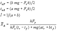
The first two terms have the dimensions of torques, that is, force by distance. It is, however, difficult to interpret them as torques on the chassis with some sort of intuitively meaningful relevance to the problem at hand. Think of them as just some expressions with interesting form extruded from the solution. The next two terms have the dimensions of inverse length. The forces, then, have the following convenient, almost pretty forms:

Finally, we can use some of MMA's graphics functions to get a visual check on these results. Apply the numerical rules to the solution for tyre 1
f1zPrototype = Simplify [nm18 [sf1z,
{}]]
(0.203749 (-17163.7 + 0.42 fx)
(-35806.2 - 0.00525
fx + 1.03068 fy)) /
(35806.2 + 0.00525 fx)
Redefine it as a function by hand so we can plot it
func1z [fx_, fy_] :=
(0.203749 *
(-17163.7 + 0.42 * fx) *
(-35806.25 - 0.00525 * fx +
1.03068 * fy))/
(35906.25 + 0.00525 * fx)
Plot3D
[func1z [x,y], {x, 0, 20000}, {y, 0, 20000}]
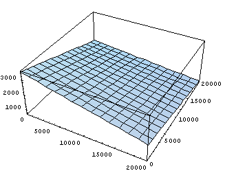
As expected intuitively, the weight on tyre 1, the right front, decreases with increasing lateral and longitudinal forces, which range from 0 to 20,000 Newtons in the plot. As the longitudinal force increases, the car is forced forward and the weight is taken off the nose. As the lateral force increases, the car is forced rightwards and weight transfers to the left as in a right-hand turn. The other three tyres behave likewise reasonably.
We have posed and solved a familiar racing problem using a programming language for symbolic mathematics. We can code up these solutions in an ordinary language like C++ and use them in our simulation program. This methodology illustrates the application of one programming language, MMA in this case, to the design of software in another programming language. In fact, there is very significant time savings in using powerful tools like this, since the alternative is coding up algebraic mistakes in C++ and then debugging them in the context of a running simulation. This latter approach is very, very time-consuming and labour-intensive. In future articles, we will use another tool, Matlab, to design some more simulation software.